Balanced System – All Workstations have equal capability e.g. 1 unmodified dice roll  – all have average capability of 3.5 units

Cadence – Frequency software is delivered to customer

Cycle – A single iteration through all Steps in the system. Sometimes called a ‘Day’. Each step has performed an action. 

Cycle Time – Amount of time the next unit in the queue is likely to take to be completed – calculated in number of cycles.

D6/Dice Roll – Refers to the result of simulating the roll of a six-sided dice  

Effort – Measure of workstation utilization, this is not correlated to effectiveness. Lower effort is time available for other activities.

Model – Series of simulations – with results averaged. 

Modifier – Ability to modify the dice roll result for a single Step, this could be positive or negative adjustments or multiple dice rolls.  

Queue – Backlog of work for the next workstation 

Simulation – We have run a set number of Cycles (likely 10 initially) This may also be referred to as a ‘Game’  

Step – A single action (dice roll) and associated events 

Throughput – Number of units delivered per cycle

WIP Limit – Work in Progress Limits: A fixed maximum number of elements permitted in a workstation. Generally used to improve flow in a system.

Workstation – Person or machine that performs a single Step 

---

Calculations:

Game View:

TOTAL WIP: Sum of all cards in workstations, excluding Backlog and Delivered.

TOTAL DELIVERED: Sum of all cards moved through the system and delivered to customers.

EST. CYCLE TIME: Estimated time (in number of cycles) for the time expected for the next card to pass fully through the system.

AVG. THROUGHPUT: Number of cards delivered divided by the number of cycles.

AVG. EFFORT: Proportion of dice roll ‘points’ that are ‘effective’ over the simulation.

Table View:

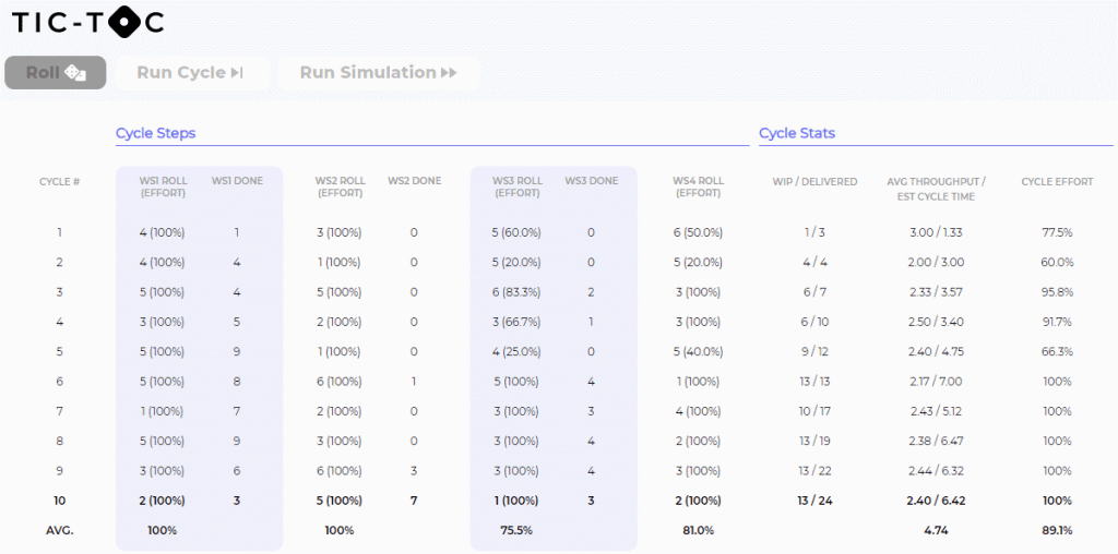
ROLL (EFFORT): The Effort indicates the % of the dice roll that is able to used. E.g. if the backlog had insufficient features, or if the WiP limit requires moving less than the dice roll.

AVG THROUGHPUT: Number of cards delivered divided by the number of cycles.

EST CYCLE TIME: Number of cards in WiP divided by the average throughput. This gives an indication of the approximate number of cycles it would take before the next card started would be completed.

CYCLE EFFORT: The total of the actual number of (modified) dice points used in activity divided by the total number of (modified) dice points rolled. This demonstrates the percentage of work lost due to dependencies, variability and imposed WiP limits. It is the utilization of resources on cards, not a reflection of efficiency.

COST OF DELAY: Each card delivered is worth one unit of value for each day in the hands of the user. The cost of delay is the loss of that value so for each day a card is completed but not delivered there is a cost of delay of one unit of value.

Model View:

In the model a simulation is run a number of times (between 500 and 10000) all of the results are averaged to eliminate statistical fluctuations to give an indicative result for the configuration.

Avg. Delivered : Number of cards delivered at the end of the simulation.

Avg. WIP : Number of incomplete cards at the end of the simulation

Avg. Throughput : Number of cards delivered divided by the number of cycles in the simulation

Avg. Effort : The total of the actual number of (modified) dice points used as activity, divided by the total number of (modified) dice points rolled.

Est. Cycle Time : Number of cards in WiP divided by the average throughput. This gives an indication of the approximate number of cycles it would take before the next card started would be completed.

Est. Delivery Time : Number of cards in WiP divided by the average throughput + 50% of the delivery cadence. This gives an indication of the approximate number of cycles it would take before the next card started would be delivered.

Est. Cost Of Delay : Each card delivered is worth one unit of value for each day in the hands of the user. If the work is ‘batched’ (delivery cadence other than daily) or there is a big bang delivery the cost of delay is the loss of that value. So for each day a card is completed but not delivered there is a ‘cost of delay’ of one unit of value.

Est. Profit: This is a projection of the simulated profit from this simulation. Project Value – Project Cost The projected value of the project is duration * daily rate * 4 expressed in dollars. The cost of the project is the daily rate * effort – cost of delay.

Est. Cost: The cost of the project is the daily rate * effort – cost of delay.

Assumptions:

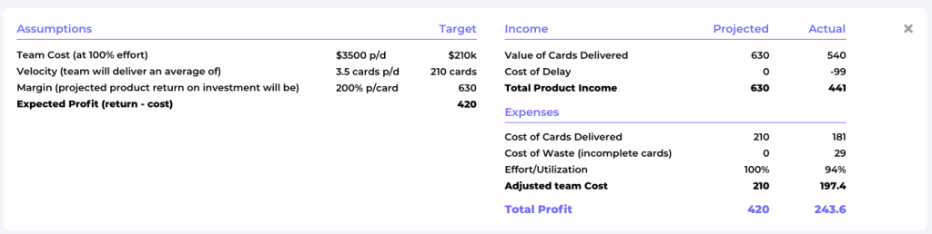
Value of a Project: Given the uncertainty and variability of software. As a very broad rule of thumb a software project should not be undertaken unless the projected value of it is considerably greater than the cost.

Lifetime of the Product: We are assuming that the lifetime of the product would be expected to be 4x the production time of the product.

Value of Cards(features): As above the value is divided by the number of cards delivered to give a value of each card.

Cost of Delivery: If we assume a team size of 7 and an approximate daily cost for the team of $3,500 this gives us a reasonable estimate for a typical agile team. The cost of delivery is the daily cost multiplied by the duration.

Cost of Delay: Each card delivered is worth one unit of value for each day in the hands of the user. The cost of delay is the loss of that value. For each day a card is completed but not delivered there is a cost of delay of one unit of value, a long delay or big bang delivery could result in a significant loss of potential income.